If you’ve done some chemistry (maybe even a bit of cheminformatics) but you’re new to machine learning, molecular solubility is a really nice first ML project: the problem is meaningful, the features are interpretable, and you can build a full pipeline without drowning in theory.

In this post, we’ll build an end-to-end machine learning pipeline that:

1. reads a dataset of molecules + measured solubility
2. turns SMILES into RDKit molecules
3. computes a small set of chemical descriptors
4. splits data into train/test sets
5. trains multiple regression models
6. evaluates them using MSE and R²
7. compares models (simple → more powerful)

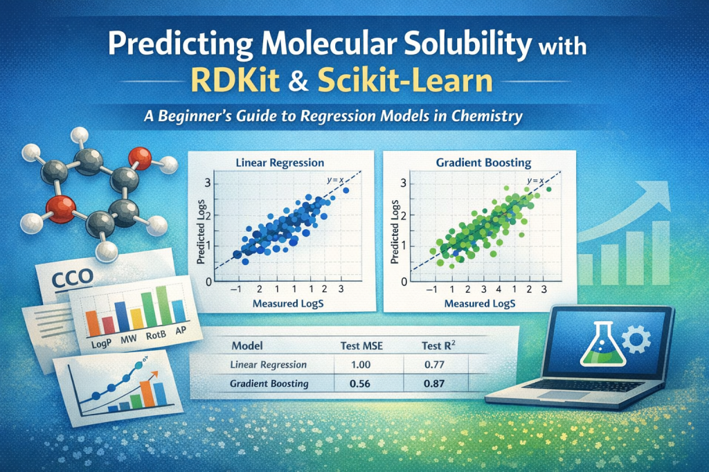
We’ll use Linear Regression as a benchmark baseline and then see why a Gradient Boosting Regressor often wins for this kind of structure-property prediction.

---

Where does this problem fit in machine learning?

Supervised learning

This is a supervised learning problem because we have:

• inputs (X): descriptors computed from molecule structures
• outputs (y): experimentally measured solubility values

The model learns a mapping from descriptors → solubility based on labeled examples.

Regression (not classification)

This is specifically a regression task because solubility is a continuous number (e.g., logS).

To contrast:

• Regression: predicts a number
  • “What is the solubility of this molecule?” → 1.23, −2.7, etc.
• Classification: predicts a category
  • “Is this molecule soluble?” → soluble / not soluble
  • or “Which solubility class?” → low / medium / high

In classification you evaluate things like accuracy or F1 score. In regression you evaluate numeric error (like MSE) and variance (like R²).

---

The dataset and our features (descriptors)

We start with a table containing at least:

• SMILES strings
• measured solubility (our target y)

Then we compute a small set of interpretable descriptors from RDKit. In the classic ESOL/Delaney style setup, a common set includes:

• MolLogP: estimated lipophilicity
• MolWt: molecular weight
• NumRotatableBonds: flexibility proxy
• Aromatic Proportion (AP): fraction of aromatic atoms in the molecule

These are not “magic ML features” – they’re chemical properties we can reason about.

---

Train/test split: why we do it

We split the dataset into:

• training set (80%): used to learn the model parameters
• test set (20%): used only at the end to evaluate how well the trained model generalizes

This is the core discipline in supervised ML: train on one set, evaluate on unseen data.

---

How we evaluate models: MSE and R²

We use two common regression metrics.

1) Mean Squared Error (MSE)

MSE measures the average squared difference between true and predicted values:$$\mathrm{MSE} = \frac{1}{n}\sum_{i=1}^{n}(y_i-\hat{y}_i)^2$$

• Lower is better.
• Squaring makes large errors hurt more (outliers matter).
• Units are “solubility units squared” (e.g., logS²), so it’s more of an optimization metric than an intuitive one.

2) Coefficient of Determination (R²)

R² answers: how much of the variance in y does the model explain compared to a dumb baseline that always predicts the mean?$$R^2 = 1-\frac{\sum_{i=1}^{n}(y_i-\hat{y}_i)^2}{\sum_{i=1}^{n}(y_i-\bar{y})^2}$$

• 1.0 is perfect.
• 0.0 means “no better than predicting the mean”.
• Negative means “worse than predicting the mean” (yes, that can happen).

How to use them together

• MSE tells you how wrong you are on average.
• R² tells you how much structure you captured in the data.

For beginner workflows, reporting both is a nice balance.

---

The models (ordered from simplest to more advanced)

We’ll go in a gentle progression: start with the simplest baseline and then try models that can represent more complex relationships.

1) Linear Regression (the benchmark)

Linear Regression assumes solubility is a weighted sum of your descriptors:$$\hat{y} = b + w_A A + w_B B + w_C C + w_D D$$

Why it’s a great beginner baseline:

• fast
• interpretable coefficients
• you can compare coefficients to literature (very satisfying in chemistry!)

It also gives you a reference point: any “fancier” model should beat this baseline on the test set to justify complexity.

2) Ridge Regression (Linear Regression + stability)

Ridge is still a linear model, but it adds a penalty for large coefficients:$$\mathrm{Loss} = \sum(y_i-\hat{y}_i)^2 + \alpha \sum w_j^2$$

This “shrinks” coefficients and can help when descriptors are correlated or noisy. Conceptually, it’s Linear Regression that’s a bit more cautious.

3) Lasso Regression (Linear Regression + feature selection)

Lasso uses a different penalty:$$\mathrm{Loss} = \sum(y_i-\hat{y}_i)^2 + \alpha \sum |w_j|$$

This can push some coefficients exactly to zero — basically doing a simple form of feature selection.

With only four descriptors, feature selection isn’t the main story, but it’s still useful to see how regularization changes behavior.

4) Elastic Net (L1 + L2 combined)

Elastic Net blends Ridge and Lasso:$$\mathrm{Loss} = \sum(y-\hat{y})^2 + \alpha\left(\rho\sum|w| + (1-\rho)\sum w^2\right)$$

• When you want some sparsity (L1) and stability (L2), Elastic Net is a nice compromise.

5) Gradient Boosting Regressor (often the winner)

Gradient Boosting is where we step beyond “one equation” and start building a model that can represent non-linear structure.

The intuition:

• you build many small decision trees (weak learners)
• each new tree tries to correct the mistakes of the previous ones
• the final prediction is a sum of these trees

This matters because molecular properties often have non-linear relationships:

• the effect of logP on solubility might depend on molecular weight
• aromaticity might matter differently depending on flexibility
• there may be thresholds, interactions, and curved trends that a straight line can’t capture

Linear regression draws a plane through descriptor space. Gradient boosting can carve up the space into regions and learn piecewise rules.

---

Why Linear Regression is the benchmark (and why Gradient Boosting often does best)

Linear Regression as a benchmark

Linear Regression is the perfect “benchmark” model because:

• it’s easy to understand
• it’s quick to train
• it gives you interpretable coefficients tied to chemistry
• it sets a baseline for performance

If a more complex model doesn’t beat it on the test set, it’s probably not worth it.

Why Gradient Boosting wins here

In solubility prediction, the relationship between a handful of descriptors and logS is rarely perfectly linear. Gradient Boosting tends to outperform because it can learn:

• non-linearity (curves, thresholds)
• feature interactions (A matters differently depending on B)
• piecewise behavior (different regimes of chemistry)

So it’s common to see:

• Linear Regression doing “pretty well” (good baseline)
• Gradient Boosting squeezing out better test performance because it can model richer relationships without you manually engineering interactions

---

What makes this an “end-to-end” pipeline?

A lot of beginner ML tutorials start at “here is X and y” and skip the chemistry part.

This pipeline is end-to-end because it includes the whole journey:

1. SMILES → RDKit molecules
2. Molecules → descriptors
3. Descriptors → train/test split
4. Training multiple models
5. Evaluating with MSE and R²
6. Comparing models and choosing the best

That’s the backbone of most real applied ML projects — not just solubility.

---

Closing thoughts

If you’re a chemist learning ML, you’re in a great position: you already understand the domain knowledge behind the data. Even a simple descriptor-based regression pipeline can teach you a ton about the ML workflow – and it’s surprisingly useful in practice.